Expedicious and Exact Extracts with Osmium

There is too much OSM data! Of course we always want more, more, more data. But when all you need is the data for your city or country, handling 34 GByte of (densly compressed) OSM data for the whole planet can be overwhelming. So one of the most often needed tools for working with OSM data is something that will cut out the region you are interested in from the huge planet file.

Or, even if you need all the data for the planet, maybe you can work on it in pieces. You can’t drive a car from Paris to New York anyway, so, if you are generating a routing graph, it makes sense to split up the worlds highways into separate pieces you can work on in isolation.

There are several tools out there that can create a geographical extract of OSM data. The oldest is Osmosis, which has to create huge temporary files to do its work making it too slow to be really useful. Much faster is Osmconvert, but it is only reasonably fast when using the special o5m format and it can only create one extract at a time. The “OSM History Splitter” can create several extracts in one go and it can, as the name implies, work on OSM history files. Originally written by Peter Körner using the old Osmium C++ library, I had ported it to the current Libosmium a while back.

All these tools solve part of the problem, but I thought I could do better. I recently released version 1.5 of the osmium-tool which has the new osmium extract command that supports everything those other tools do and is faster and easier to use than any of them.

Lets look at some of the problems involved in creating extracts of OSM data:

First you have to read and write OSM files quickly. If you want to split up the planet into, say, several continent-sized extracts, you have to read 34 GBytes of data from one file and write about the same amount to several other files. Libosmium has gotten really fast at that, because it is using multithreading. (Someday I have to write about that some more.)

Second, you have to figure out which objects from the input should end up in which output file. The OSM nodes contain locations and you have to figure out whether those coordinates are inside the region you are interested in or not. Sometimes the region is specified as a bounding box. That is easy and fast then, a maximum of four comparisons and you know whether a location is inside or not. But often you want to cut out a more irregular shape. For this you need what’s called a point-in-polygon algorithm, that tells you whether a location is inside a given polygon. There are several well-known point-in-polygon algorithms, the simplest one is the “crossing number algorithm”. Simply count how often an imaginary ray from the point to infinity crosses the polygon boundary. If the number of crossings is odd, the point is inside, if the number is even, the point is outside.

This algorithm needs at most O(n) time to check one point, because it has to check each point against each of the “segments” in the polygon boundary. For polygons with many segments, this can be hugely expensive. There are many ways to break this down and make it more efficient. The one I used is still pretty simple and turns out to be fast enough that the point-in-polygon algorithm isn’t the bottleneck in this program any more.

Before doing the point-in-polygon checks we split up the polygon into equally sized “horizontal bands” (one band shown in red in the image). For each band we create a list of segments that cross this band (the red segments in the image). Now for each location of a node we find the band it is in (a simple calculation) and only check against all the segments in this band. How many bands do we use? Some experimentation shows that having about 10-20 segments in a band gives good enough performance, fewer segments don’t improve it much. So we devide the number of segments in the polygon by 10 and use that as the number of bands.

All of this is done in the program without using any library which allows us to do the point-in-polygon check without any memory-managment overhead or something like it often associated with library use. The OSM History Splitter uses the GEOS library for this which has a clever implementation but so much overhead that it is much more expensive. Doing all of this ourselves even allows the whole thing to be done with integers alone, avoiding the more expensive floating point operations, because we have the coordinates as integers anyway and can make sure that there can be no overflow. (Did you wonder why the “rays” are going to the left and not the top or bottom? For the algorithm it doesn’t matter in which direction they go, but because the x-coordinates are between -180 and 180, but the y coordinates are only between -90 and 90 some calculations will always fit into a 32 bit integer this way.) In the end the code isn’t even 200 lines including all the comments.

This solves the problem which nodes should end up in which extract. But OSM is more than nodes. There are those pesky ways and relations which don’t have a location but only refer to the nodes which do. So we have to figure out what belongs to what and this is not straightforward. Do we want the complete ways even if they cross the boundary of our region? Which relation members do we need? There is no one-size-fits-all solution for this, because it depends on what you want to do with the data. All other programs implement different options for this case and Osmium does too. It offers three strategies: The “simple” strategy, the “complete_ways” strategy and the “smart” strategy. They differ in what they extract, how often they need to read the input file for this and how much memory they need. Instead of describing them here I refer the reader to the manual. As it turns out even the most expensive strategy, the “smart” strategy, which needs to read the input file three times, runs in reasonable time due to the well optimized file reader in Libosmium. The big advantage of the smart strategy is that all multipolygons crossing the boundary of your region will be completely in the output.

Here are some numbers comparing the strategies: Reading the planet file and creating six extracts for the continents using rough polygons is done in about 16 minutes with the “simple” strategy, in slightly less then 20 minutes with the “complete_ways” strategy, and in about 21 minutes with the “smart” strategy. (All numbers in this post are benchmarked on a 4 core Intel Xeon CPU E3-1275 v5 @ 3.60GHz with hyperthreading, 64GB RAM, and NVRAM SSD.)

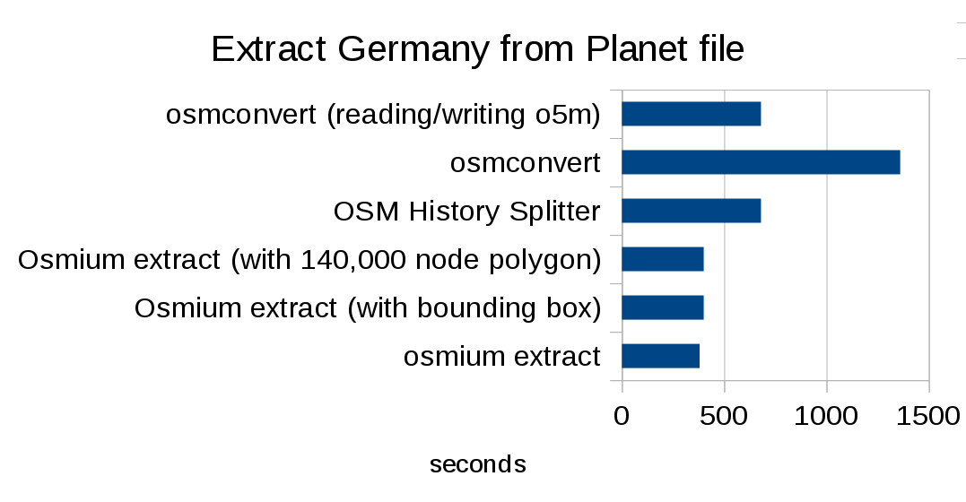
The bottleneck is not the reading of the file or the point-in-polygon, the bottleneck here is the writing of the PBF files which is not optimized as well as the reading. If you only cut out a Germany polygon from the planet, the “complete_ways” runs in about 380 seconds, it has to read the same amount of data as above, but much less to write. Using a bounding box instead of a polygon slows this to about 400 seconds, because there is more data to write. But in any case this is much faster than the OSM history splitter (about 680 seconds) and osmconvert (1360 seconds). (If you use the o5m format, osmconvert can do this in 680 seconds, because the format is more efficient to read, but the file size is much bigger than PBF.) Note that it doesn’t matter much whether you are using a simplified polygon or, for instance, the full Germany boundary from OSM (with more than 140,000 nodes), the way the algorithm is implemented makes this fast enough (a bit less than 400 seconds).

So the new tool is much faster than all the alternatives, but it is also easier to use. You can either specify the region to extract on the command line, or, especially if you have multiple regions you want to extract in one go, use a config file. Regions can be extracted by bounding box or polygon and there are multiple ways to specify those polygons, including GeoJSON, the poly format, or as an OSM file with a (multi)polygon in it. In fact writing all the code for those file parsers, checking the command line options, and giving helpful error messages if something went wrong etc. took much longer than writing the algorithm itself. But that is part of writing a useful tool, too.

Most of you are probably aware of the OSM extracts that the Geofabrik creates daily and offers for download. As probably the most heavy “creator” of extracts I gave a pre-release version of Osmium to Frederik Ramm to test out. He found a few bugs which I fixed (thanks!). And he was so impressed by the speedups that he brought the released version immediately into production. He writes on the Geofabrik Blog: “Using the new software has also brought down the overall processing time from around 10 hours to under 4 hours…” (Not all of that is the extract creation itself, but some other changes due to the use of Osmium.)

Osmium version 1.5.1 is available now. Packages for Debian and other distributions are available. There is a manual and extensive man pages describing every option and detail. Try out osmium-extract and all the other things the Osmium tool has to offer.